Up: Class 6, Math 696
Next: Homework
Previous: Activities
More about graphics with Maple
You are familiar with Maple's capabilities for symbolic
calculation: Maple can differentiate and integrate functions, factor
polynomials, and so on. You also know about Maple's numerical
capabilities: Maple can do floating point arithmetic, find
numerical approximations to solutions of equations, do numerical
integration, and so on.
However, the ``knock your socks off'' applications of modern
computer technology are the pretty pictures you can make. It is
computer graphics that made ``fractal'' a household word. Last
time we played with some two-dimensional plots. Today we will go
further. (We will also see why the pictures are useful.)
Open up a Maple window, and before you do anything else,
remember to load the plots package via the
with(plots): command. Recall that section 2.4 of the
CalcLabs
with Maple V manual summarizes some of Maple's basic
plot commands. In addition, I have made a summary of Maple's
two-dimensional plot commands for quick
reference.
A sneaky problem for review
For review, try the following problem from Benny Evans and Jerry
Johnson, Uses of Technology in the Mathematics
Curriculum, as quoted in George B. Thomas and Ross L.
Finney, Calculus, eighth edition, page 235:
Find the
local extrema and inflection points of the graph of the function
f(x) = (1/8)x8 -
(1/2)x6 - x5 +
5x3.
This function is a simple polynomial, but the computer is going
to mislead you unless you pay attention to the questions you ask it.
Suggestions:
Polar coordinates
 Next read through pages 121-123 (Chapter
12) of the CalcLabs with Maple V manual (about
plotting parametrized curves and polar equations). Then make a
plot of the lemniscate
that is described in polar coordinates in LaTeX notation by
$r^2 = \sin 2\theta$. This is not so easy! What is
a good way to handle the squared term?
Now make your lemniscate fancier.
Try using some of the following plot options:
scaling=constrained
numpoints=100
title=`lemniscate`
thickness=3
linestyle=2
titlefont=[HELVETICA,OBLIQUE,36]
view=[-1..1,-1..1]
color=COLOR(RGB, 0.1960, 0.6000, 0.8000)
What do all these options do?
You can learn more about plot options from the on-line help via
the command ?plot[options].
Here is another way to dress up the plot: superimpose
it on a colored background. Define your lemniscate plot as
plot1 and then use the command
plot2 := polygonplot([
[-2,-2], [2,-2], [2,2], [-2,2]], color=cyan, axes=none):
to define a colored square. Now try
display([plot1,plot2]); to view your plot on a
cyan background.
Fun and games with animation
Before we go on to three-dimensional plots, let's play a
little game with Maple's animation feature. Have you seen those
screen savers that bounce a geometric figure around the screen?
You can create a similar effect with Maple.
Enter the following code in Maple (you can cut and paste it with
the mouse):
r1:=rand(-10..10):  r2:=10^(-12)*rand:
p:=seq(plots[polygonplot]([[r1(),r1()],[r1(),r1()],[r1(),r1()]],
             color=COLOR(RGB, r2(), r2(), r2() ) ), i=1..100):
plots[display]([p], insequence=true, axes=none,
           title=`Moving Triangles`, titlefont=[TIMES,BOLD,72]);
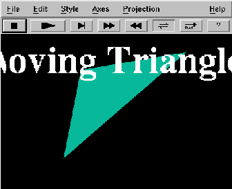 A plot window should pop up that looks something like the figure.
Click on the question mark button to get an explanation of what
the other buttons do. Click on the ``Playback Mode'' button to
change it to a loop, maximize the plot window, and click on the
``Play'' button. You should get a display of moving colored
triangles. The display continues until you click on the ``Stop''
button. There are buttons to adjust the speed of the playback.
Explanation: Maple's rand command is a random number
generator. By default, it produces pseudo-random 12-digit
non-negative integers. Thus, the r2 function defined
above generates a random rational number between 0 and 1. The
color instruction above generates a color with a
random mixture of Red, Green, and Blue. The command
rand(-10..10) produces a random integer between -10
and 10, so the polygonplot command above makes a
triangle whose vertices are at random integer points within a 20
by 20 square. The whole procedure generates a sequence of 100
randomly placed triangles with random colors, and the
insequence=true command produces the animation.
Three dimensional plots
Now let's look at some examples of three-dimensional plots.
Start with something simple, like
plot3d(x^2+y^2,x=-2..2,y=-2..2); to generate the
graph of a paraboloid.
Notice that there are many options on the plot window. By holding down
the left mouse button, you can drag the plot to a new
orientation; then click the middle mouse button to redraw the
plot. The ``Axes'' menu lets you choose different styles for the
coordinate axes (normal, boxed, framed, or none). The
color menu gives options for different color and lighting
schemes, and the Style menu selects different ways to draw the
surface (patches, grids, and so on).
Try adding some of the following options to the plot3d command:
title=`paraboloid`,titlefont=[TIMES,ROMAN,24]
shading=Z
thickness=2
axes=BOXED
style=PATCHNOGRID
color=x*y
projection=FISHEYE
Maple can plot implicitly defined surfaces. You can get a
sphere of radius 2 via implicitplot3d(x^2+y^2+z^2=4,
x=-2..2, y=-2..2, z=-2..2, scaling=constrained); for
example.
Alternatively, a sphere can be constructed as a parametric
surface. For a two-dimensional surface, we need two parameters,
say s and t. Try
plot3d( [2*sin(s)*cos(t), 2*sin(s)*sin(t), 2*cos(s)],
s=0..Pi, t=0..2*Pi, scaling=constrained);
for example.
What do s and t represent in spherical
coordinates?
Maple knows about polar coordinates in two dimensions, and it
knows about spherical coordinates in three dimensions. The
command sphereplot(2, theta=0..2*Pi, phi=0..Pi,
scaling=constrained); is yet another way to plot a sphere.
A new feature appears in three dimensions that we did not see
in two dimensions. Since there is more room in three dimensions,
we have the possibility of plotting either a two-dimensional
surface or a one-dimensional curve. We just saw above how to plot
a surface. To plot a one-dimensional parametrized curve, use the
spacecurve command. For example, spacecurve(
[cos(t), sin(t), t], t=0..4*Pi, title=`helix`); plots a
helix.
A common way to describe a three-dimensional object is to specify
its cross section at each point along a curve. For example, a
cylinder is simply the Cartesian product of a line with a circle.
Maple has a tubeplot command that implements this
idea. For example, tubeplot( [cos(t), sin(t), t],
t=0..4*Pi, radius=0.5, tubepoints=30, title=`helix tube`);
draws a tube of
constant radius around the helix. What happens if you
set radius=t/6 and scaling=constrained?
Who cares?
Did you enjoy playing with the pictures?
Is there some importance to making pretty pictures besides the
recreational aspect? I think so.
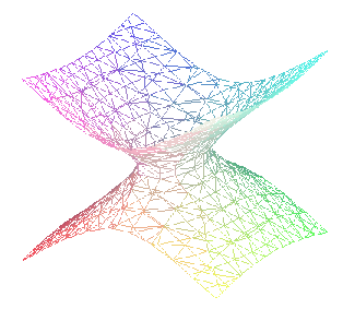 The cliché ``a picture is worth a thousand words'' has a lot
of truth to it, because many (most?) people are visual thinkers.
If you shake me awake at three o'clock in the morning and demand,
``Define a hyperboloid of one sheet,'' I probably will not give you
a very coherent answer. If instead you say, ``Describe the surface
with equation x2 + 3y2 -
5z2 = 1,'' I may do a little
better. If you give Maple the command
 implicitplot3d(
x^2+3*y^2-5*z^2=1, x=-2..2, y=-2..2, z=-2..2,
orientation=[30,70], grid=[10,10,20],
scaling=constrained); to produce the figure, then
you will be more satisfied.
Putting Maple graphics into Web pages
Suppose you have created a wonderful plot with Maple, and you
would like to share it with the world by putting it on your home
page on the World-Wide Web. How can you do this?
First you need to turn the Maple plot into a graphics file in
either gif or jpeg format. There are
several ways to do this.
-
With Maple V Release 3.
Have Maple display a plot, then on the ``File'' menu
on the plot window choose the ``Print'' option. We used this
option previously to capture graphics to a PostScript file to
include in LaTeX documents. Instead of selecting ``Postscript''
from the menu, select ``GIF.'' Then Maple
will write the plot out to disk in gif
format. Alternatively, execute the Maple command
plotsetup(plotdevice=gif,plotoutput=`myplot.gif`);
and then your plot will be written directly to a graphics
file. The command plotsetup(x11); will restore the
default behavior of displaying plots in separate windows.
-
With Maple V Release 4.
The new release of Maple no longer supports gif
format, due to copyright concerns. Instead, Maple V Release 4 can
write out jpeg files. Use the command
plotsetup(plotdevice=jpeg,plotoutput=`myplot.jpeg`);
to use this feature; restore the default behavior via the
plotsetup(default); command.
With xv. The program xv is
a graphics viewer for x-windows. If you do not find it on
the root menu, start it from a terminal window with the
command ``xv &.'' By default, xv starts up with
its control panel hidden; click the right mouse button in
the xv window to bring up the control panel.
Click the ``Grab'' button on the xv
control panel. Then hold down the middle mouse button and
drag the mouse to draw a cropping rectangle on the screen
(around your favorite plot, for example). When you let the
mouse button up, xv will grab a copy of that rectangular
area. Then use the ``Save'' button on the xv
control panel to save your image in one of a choice of
graphics formats (either gif or
jpeg is good for Web pages).
The program xv can also convert between
different image formats, and it can write (but not read)
PostScript files for inclusion into LaTeX documents. You
can use the ``ColEdit'' button to change the
colors of images (for instance, to change the background
color).
Once you have saved your image in graphics format, you get it
onto your home page the same way as in Class
3. Namely, make the image world-readable by issuing the command
chmod a+r filename in a terminal window,
and move it into your public_html directory via the
command mv filename
public_html/filename. (Or you can move the
file via ``drag and drop'' with the xdir file manager;
or in emacs, use ``Open directory'' on the ``Files''
menu, and then use the ``Operate'' menu.) Then open your
public_html/index.html file in a text editor, and
insert something like this:
<p>Here is an image I created with Maple. <img src="myplot.gif">
</p>
Bring up your home page and see if the image appears.
The HTML image tag ``img'' takes several
arguments. The src="ImageName" argument specifies
the URL of the source image. If you have found a nice image at a
remote site, and you do not want to store a copy locally, you can
link the remote image into your page by specifying the remote URL
as the source. For example, the code <img
src="https://www.nd.edu/StudentLinks/akoehl/Pascal.gif">
will pull a remote picture of Blaise Pascal into your Web page.
The optional argument ALIGN controls how the image
lines up with surrounding text. You can say <img
src="ImageName" align=TOP> to make text line up with
the top of the image. (Other values are CENTER and
BOTTOM.) Some browsers support
align=right and align=left, which wrap
text around the image. (Mosaic does not support this option yet.)
Another useful option is alt="some
text". Non-graphical browsers like lynx will
display ``some text'' in place of the image. Some graphical
browsers will display the alternate text temporarily while they
are downloading the image. You can speed up page loading for some
browsers by specifying the size of the image in pixels via
WIDTH=number and HEIGHT=number. (You
can find out the size of the image from the xv
program, for instance.)
By the way, links to non-graphical items on the Web use the
``A'' tag, following a
similar syntax to the ``img'' tag. The following HTML
code is a link to the home page of the Department of Mathematics at
Texas A&M University.
<A href="/">TAMU Math</A>
The browser will display this as TAMU Math underlined or in color.
Up: Class 6, Math 696
Next: Homework
Previous: Activities
Comments to Harold P.
Boas.
Created Oct 9, 1996.
Last modified Oct 9, 1996.
 Next read through pages 121-123 (Chapter
12) of the CalcLabs with Maple V manual (about
plotting parametrized curves and polar equations). Then make a
plot of the lemniscate
that is described in polar coordinates in LaTeX notation by
 A plot window should pop up that looks something like the figure.
Click on the question mark button to get an explanation of what
the other buttons do. Click on the ``Playback Mode'' button to
change it to a loop, maximize the plot window, and click on the
``Play'' button. You should get a display of moving colored
triangles. The display continues until you click on the ``Stop''
button. There are buttons to adjust the speed of the playback.
 The cliché ``a picture is worth a thousand words'' has a lot
of truth to it, because many (most?) people are visual thinkers.
If you shake me awake at three o'clock in the morning and demand,
``Define a hyperboloid of one sheet,'' I probably will not give you
a very coherent answer. If instead you say, ``Describe the surface
with equation x2 + 3y2 -
5z2 = 1,'' I may do a little
better. If you give Maple the command