Up: Activities
Next: Homework
Previous: Discussion

Introduction to programming in Maple

First work through section 13.1 (pages 127-131) of the CalcLabs with Maple V manual. The manual introduces the notion of a Maple procedure. It also illustrates a simple do loop.

The 3x+1 problem

Another standard programming construct is if ... then ... else. Here is an example of a Maple if statement.

     Collatz:=proc(n)
       if type(n,even) then n/2;
       else 3*n+1;
       fi;
     end;

This Maple code defines a function named Collatz of one argument n that sends n into n/2 if n is even, and sends n into 3n+1 if n is odd. (The procedure could be improved by including a check to see if n is an integer, and issuing an error message if it is not.)

There is a famous unsolved problem---sometimes called the 3x+1 problem---about the iterates of the Collatz function. Is it the case that for every positive integer n, when you apply the function repeatedly you eventually fall into the cycle 1->4->2->1?

For example, if you start with the number 25, successive applications of the function lead to the sequence 25, 76, 38, 19, 58, 29, 88, 44, 22, 11, 34, 17, 52, 26, 13, 40, 20, 10, 5, 16, 8, 4, 2, 1. No one knows if you eventually end up at 1 from an arbitrary starting point. For more about this problem, see a paper by Jeff Lagarias.

Here are two exercises to work in class to get practice with Maple procedures.

Exercise for groups 1 and 3

Write a Maple procedure that takes one argument and returns the number of iterations of the Collatz function required to reach the value 1 from the given starting point (assuming, of course, that the number of iterations is finite).

Exercise for groups 2 and 4

Write a Maple procedure that takes one argument and determines the largest number attained by repeatedly applying the Collatz function to that value (assuming, of course, that there is such a largest number).

Fractals

Here is an example of a somewhat more elaborate Maple procedure. It plots a fractal image constructed by the iterated function scheme discussed by Michael Barnsley in his book Fractals Everywhere, Academic Press, 1988 (see especially section 3.8). Thanks to Simon Rentzmann, who included an example similar to this in his class project for fall 1995.

After the code is an explanation of what it does. You can try cutting the code with the mouse and pasting it into a Maple session. If you then execute the command fractal(100); you should get 100 points of a fractal image. (The plot starts to look recognizable with about 400 points.)

fractal:=proc(n)
local Mat1, Mat2, Mat3, Mat4, Vector1, Vector2, Vector3, Vector4,
Prob1, Prob2, Prob3, Prob4, P, prob, counter, fractalplot;
Mat1:=linalg[matrix]([[0.0,0.0],[0.0,0.16]]);
Mat2:=linalg[matrix]([[0.85,0.04],[-0.04,0.85]]);
Mat3:=linalg[matrix]([[0.2,-0.26],[0.23,0.22]]);
Mat4:=linalg[matrix]([[-0.15,0.28],[0.26,0.24]]);
Vector1:=linalg[vector]([0,0]);
Vector2:=linalg[vector]([0,1.6]);
Vector3:=linalg[vector]([0,1.6]);
Vector4:=linalg[vector]([0,0.44]);
Prob1:=0.01; 
Prob2:=0.85;
Prob3:=0.07;
Prob4:=0.07;
P:=linalg[vector]([0,0]);
readlib(readdata):   readlib(write):
   # omit the previous line for Maple V Release 4
print(time());
open(fractaldata);
   # omit the previous line for Maple V Release 4
for counter from 1 to n do
   prob:=rand()/10^12;
   if prob<Prob1 then P:=evalm(Mat1&*P+Vector1)
       elif prob<Prob1+Prob2 then P:=evalm(Mat2&*P+Vector2)
           elif prob<Prob1+Prob2+Prob3 then P:=evalm(Mat3&*P+Vector3)
              else P:=evalm(Mat4&*P+Vector4);
   fi;
   writeln(P[1],P[2]);
     # for Maple V Release 4, change the previous line to
     # writedata[APPEND](fractaldata, [[P[1],P[2]]], [float,float]);
od;
close();
     # for Maple V Release 4, change the previous line to
     # fclose(fractaldata); 
fractalplot:=readdata(fractaldata,2);
print(plot(fractalplot, style=point, scaling=constrained,
           axes=none, color=green, title=``.n.` iterations`));
print(time());
end;

fern The mathematics underlying this code is the following iteration scheme. Pick a vector in the plane and apply an affine transformation (multiply by a matrix and add some vector to the result). Plot the resulting point. Apply to the new point a possibly different affine transformation. Repeat. In the given example, there are four different affine transformations involved, and the one that is picked at a given step is randomized; each transformation has a specified probability of being chosen at any particular step.

The final plot is thus a set of points in the plane, and because of the randomness, a different set each time the procedure is executed. The surprise is that for a large number of iterations, the final picture always looks the same.

This particular example is a fractal fern, shown in the illustration for a large number (25,000) of iterations. Maple took about 17 minutes to compute this picture. I changed the final plot to display points as dots instead of crosses. (Crosses show up better when a small number of points is plotted.)

Notice the self-similarity typical of fractals. Each leaf of the fern looks like a copy of the whole fern.

Now let's see what the Maple code does.

fractal:=proc(n): This line defines fractal to be the name of a procedure that takes one argument n.
local Mat1, Mat2, ...: This defines a number of variables that are local to the procedure. The same names could be used for other variables outside the procedure with no conflict.
Mat1:=linalg[matrix]([[0,0],[0,0.16]]);: The next section of code specifies values for some of the local variables. The variable Mat1 is a 2x2 matrix. The matrix function is part of the linear algebra package; it could be called by the name matrix instead of linalg[matrix] if we first loaded the package via with(linalg):. The next few lines of code set values for the other three matrices, for the four constant vectors in the affine transformations, for the probabilities of choosing each affine transformation, and for the initial point.
readlib(readdata): readlib(write):: This line loads Maple functions for reading data from disk files and writing data to disk files.
print(time());: This instruction prints the amount of computation time so far during the Maple session. There is a second copy of this instruction at the end of the procedure. By subtracting, you can determine how long the procedure takes to execute.
open(fractaldata);: This opens a disk file named fractaldata for writing. If the file does not exist, Maple will create it.
for counter from 1 to n do: This starts a loop that is terminated by od;.
prob:=rand()/10^12;: Maple's rand function generates a pseudo-random 12-digit non-negative integer. Dividing by 10¹² gives a random probability between 0 and 1.
if prob<Prob1 then P:=evalm(Mat1&*P+Vector1): The if ... fi; section of code that starts here says to apply one of the four affine transformations to the point P, and then relabel P as this new point. Which transformation is chosen depends on the value of the random probability determined above.
writeln(P[1],P[2]);: This writes the two coordinates of the point P to the previously opened disk file.
close();: This closes the disk file.
fractalplot:=readdata(fractaldata,2);: Here we read the data in the disk file and store the whole list in fractalplot.
print(plot(fractalplot, ...: Now we tell Maple to construct the plot of the data and to display the plot.
print(time());: Comparing to the starting time shows how long it took Maple to execute the procedure. (Maple is relatively slow at executing a program of this nature.)

Exercise

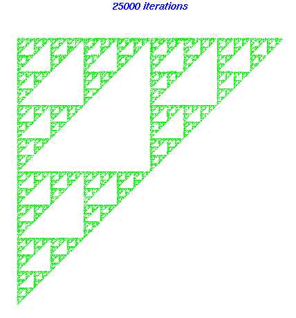
Construct a Sierpinski triangle by a similar algorithm. Use three affine transformations with equal probabilities. Each transformation has the same matrix matrix([[0.5,0.0],[0.0,0.5]]);, but the vectors are [0,0], [0,10], and [10,10].

sierpinski
triangle Your picture should look something like the figure.

Up: Activities
Next: Homework
Previous: Discussion