I had fun seeing what interesting Internet resources you turned up. Here are some of them:
Discussion of what lessons can be learned from the oral presentations of last week:
By the way, the presentations were excellent!
Today you are going to expand your knowledge of Maple's graphics capabilities.
You are familiar with Maple's capabilities for symbolic calculation: Maple can differentiate and integrate functions, factor polynomials, and so on. You also know about Maple's numerical capabilities: Maple can do floating point arithmetic, find numerical approximations to solutions of equations, do numerical integration, and so on.
However, the "knock your socks off" applications of modern computer technology are the pretty pictures you can make. It is computer graphics that made "fractal" a household word. So today let's crank up Maple and make some pretty pictures. (We will also see why the pictures are useful.)
Open up a Maple window, and before you do anything else,
remember to load the plots package via the
with(plots): command. Recall that section 2.4 of the
CalcLabs with Maple V manual summarizes some
of Maple's basic plot commands.
For review, try the following problem from Benny Evans and Jerry
Johnson, Uses of Technology in the Mathematics
Curriculum, as quoted in George B. Thomas and Ross L.
Finey, Calculus, eighth edition, page 235: Find the
local extrema and inflection points of the graph of the function
that is
given in Maple notation by f:= x^8/8 -x^6/2 -x^5 +5*x^3.
This function is a simple polynomial, but the computer is going
to mislead you unless you pay attention to the questions you ask it.
Suggestions:
Next read through pages 121-123 (Chapter 12) of the
CalcLabs with Maple V manual (about plotting
parametrized curves and polar equations). Then make a plot of
the lemniscate that is described in polar coordinates in LaTeX
notation by $r^2 = \sin 2\theta$. This is not so easy!
What is a good way to handle the squared term?
Now make your lemniscate fancier. Try using some of the following plot options:
scaling=constrained
numpoints=100
title=`lemniscate`
thickness=3
linestyle=2
titlefont=[HELVETICA,OBLIQUE,36]
view=[-1..1,-1..1]
color=COLOR(RGB, 0.1960, 0.6000, 0.8000)
What do all these options do?
You can learn more about plot options from the on-line help via
the command ?plot[options].
Here is another way to dress up the plot: superimpose
it on a colored background. Define your lemniscate plot as
plot1 and then use the command
plot2 := polygonplot([
[-2,-2], [2,-2], [2,2], [-2,2]], color=cyan, axes=none):
to define a colored square. Now try
display([plot1,plot2]); to view your plot on a
cyan background.
Before we go on to three-dimensional plots, let's play a little game with Maple's animation feature. Have you seen those screen savers that bounce a geometric figure around the screen? You can do something similar with Maple.
This exercise is going to stress the capabilities of your color terminal. If you have Netscape open, you had better close it (or you will probably run out of memory).
Enter the following code in Maple (you can cut and paste it with the mouse):
r1:=rand(-10..10):  r2:=10^(-12)*rand:
p:=seq(plots[polygonplot]([[r1(),r1()],[r1(),r1()],[r1(),r1()]],
                 color=COLOR(RGB, r2(), r2(), r2() ) ), i=1..100):
plots[display]([p],insequence=true,axes=none,title=`Moving Triangles`,
                titlefont=[TIMES,BOLD,72]);
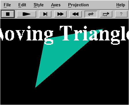
A plot window should pop up that looks something like this:

Click on the question mark button to get an explanation of what the other buttons do. Click on the "Playback Mode" button to change it to a loop, maximize the plot window, and click on the "Play" button. You should get a display of moving colored triangles. The display continues until you click on the "Stop" button. There are buttons to adjust the speed of the playback.
Explanation: Maple's rand command is a random number
generator. By default, it produces pseudo-random 12-digit
non-negative integers. Thus, the r2 function defined
above generates a random rational number between 0 and 1. The
color instruction above generates a color with a
random mixture of Red, Green, and Blue. The command
rand(-10..10) produces a random integer between -10
and 10, so the polygonplot command above makes a
triangle whose vertices are at random integer points within a 20
by 20 square. The whole procedure generates a sequence of 100
randomly placed triangles with random colors, and the
insequence=true command produces the animation.
plot(x^4+sin(Pi*x),x=-1..1);
y=x^4+sin(Pi*x) for
x between -1 and 1.
implicitplot(x^2+y^2=1,x=-1..1,y=-1..1);
x^2+y^2=1.
plot( [cos(t), sin(t), t=0..2*Pi] );
x=cos(t) and y=sin(t).
polarplot(1, t=0..2*Pi);
r=1.
display( [plot1, plot2] );
plot1 and
plot2 together. (There is also an
animate command.)
plot( [ [1,2], [-3,4], [5,6] ] );
(1,2) to the point (-3,4) and
the second from the point (-3,4) to the point
(5,6).
polygonplot( [ [1,2], [-3,4], [5,6] ] );
(1,2),
(-3,4), and (5,6).
axes=NONE
axes are NORMAL,
FRAMED, and BOXED.
scaling=CONSTRAINED
UNCONSTRAINED.
numpoints=100
color=red
title=`Bonfire`
Now let's look at some examples of three-dimensional plots.
Start with something simple, like the paraboloid:
plot3d(x^2+y^2,x=-2..2,y=-2..2);
Notice that there are many options on the plot window. By holding down the left mouse button, you can drag the plot to a new orientation; then click the middle mouse button to redraw the plot. The "Axes" menu lets you choose different styles for the coordinate axes (normal, boxed, framed, or none). Try it. The color menu gives options for different color and lighting schemes, and the Style menu selects different ways to draw the surface (patches, grids, and so on).
Try adding some of the following options to the plot3d command:
title=`paraboloid`,titlefont=[TIMES,ROMAN,24]
shading=Z
thickness=2
axes=BOXED
style=PATCHNOGRID
color=x*y
projection=FISHEYE
Maple can plot implicitly defined surfaces. You can get a sphere
of radius 2
via
implicitplot3d(x^2+y^2+z^2=4, x=-2..2, y=-2..2, z=-2..2,
scaling=constrained);
for example.
Alternatively, a sphere can be constructed as a parametric
surface. For a two-dimensional surface, we need two parameters,
say s and t. Try
plot3d( [2*sin(s)*cos(t), 2*sin(s)*sin(t), 2*cos(s)],
s=0..Pi, t=0..2*Pi, scaling=constrained);
for example.
What do s and t represent in spherical
coordinates?
Maple knows about polar coordinates in two dimensions, and it
knows about spherical coordinates in three dimensions. The command
sphereplot(2, theta=0..2*Pi,
phi=0..Pi, scaling=constrained);
is yet another way to
plot a sphere.
A new feature appears in three dimensions that we did not see
in two dimensions. Since there is more room in three dimensions,
we have the possibility of plotting either a two-dimensional
surface or a one-dimensional curve. We just saw above how to plot
a surface. To plot a one-dimensional parametrized curve, use the
spacecurve command. For example, spacecurve(
[cos(t), sin(t), t], t=0..4*Pi, title=`helix`); plots a
helix.
A common way to describe a three-dimensional object is to specify
its cross section at each point along a curve. For example, a
cylinder is simply the Cartesian product of a line with a circle.
Maple has a tubeplot command that implements this
idea. For example, tubeplot( [cos(t), sin(t), t],
t=0..4*Pi, radius=0.5, tubepoints=30, title=`helix tube`);
draws a tube of
constant radius around the helix. What happens if you
set radius=t/6 and scaling=constrained?
Did you enjoy playing with the pictures? Is there some importance to making pretty pictures besides the recreational aspect? I think so.
The cliché "a picture is worth a thousand words" has a lot
of truth to it, because many (most?) people are visual thinkers.
If you shake me awake at three o'clock in the morning and demand,
"Define a hyperboloid of one sheet", I probably will not give you
a very coherent answer. If instead you say, "Describe the surface
with equation x^2+3*y^2-5*z^2=1", I may do a little
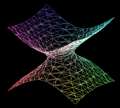
better. If you give Maple the command implicitplot3d(
x^2+3*y^2-5*z^2=1, x=-2..2, y=-2..2, z=-2..2,
orientation=[30,70], grid=[10,10,20],
scaling=constrained); and get the following picture, then
you will be satisfied.

The surprise is that a square appears in the solution of this problem!
Your task is to write (in LaTeX) an explanation and solution of this problem (addressed to an audience of calculus students). Include some graphics, since a big part of the problem is to visualize the region. There are several ways to set up an integral for the volume; pick the one that you think is simplest. You may use Maple to compute the integral, if you wish.
Hint about the graphics: the square should pop out at you if you use
the plot option style=contour.
If you have not started, don't panic, but you do need to do some serious thinking about the projects.
We spent some time in class working on World-Wide Web home pages, so you should have a good start on Project A. Remember that part of the project is to help someone else with a home page. (One possibility is to look at the Mathematics Faculty Directory, pick a professor with a minimal home page, and help improve the page.)
You may be interested in looking at the home pages of other students in the class.
Concerning a second project (either project B or project C), what I would like to see by October 20 is an outline: what is the topic, what do you plan to do, what are some resource materials that you have located.